CM Topologies - Part 1
I want to start a series of post discussing CM systems (controller-model systems).
CM systems are the subject of this paper: On Learning to Think: Algorithmic Information Theory for Novel Combinations of Reinforcement Learning Controllers and Recurrent Neural World Models. The discussion really takes off in section 5: (C is the controller and M the model)
5 The Controller C Learning to Exploit RNN World Model M
5.1 C as a Standard RL Machine whose States are M’s Activations . . . . . . . . . . . 12
5.2 C as an Evolutionary RL (R)NN whose Inputs are M’s Activations . . . . . . . . . .12
5.3 C Learns to Think with M: High-Level Plans and Abstractions . . . . . . . . . . . . . 12
5.4 Incremental / Hierarchical / Multitask Learning of C with M . . . . . . . . . . . . . . . .14
I’ll include the figure shown in the paper:
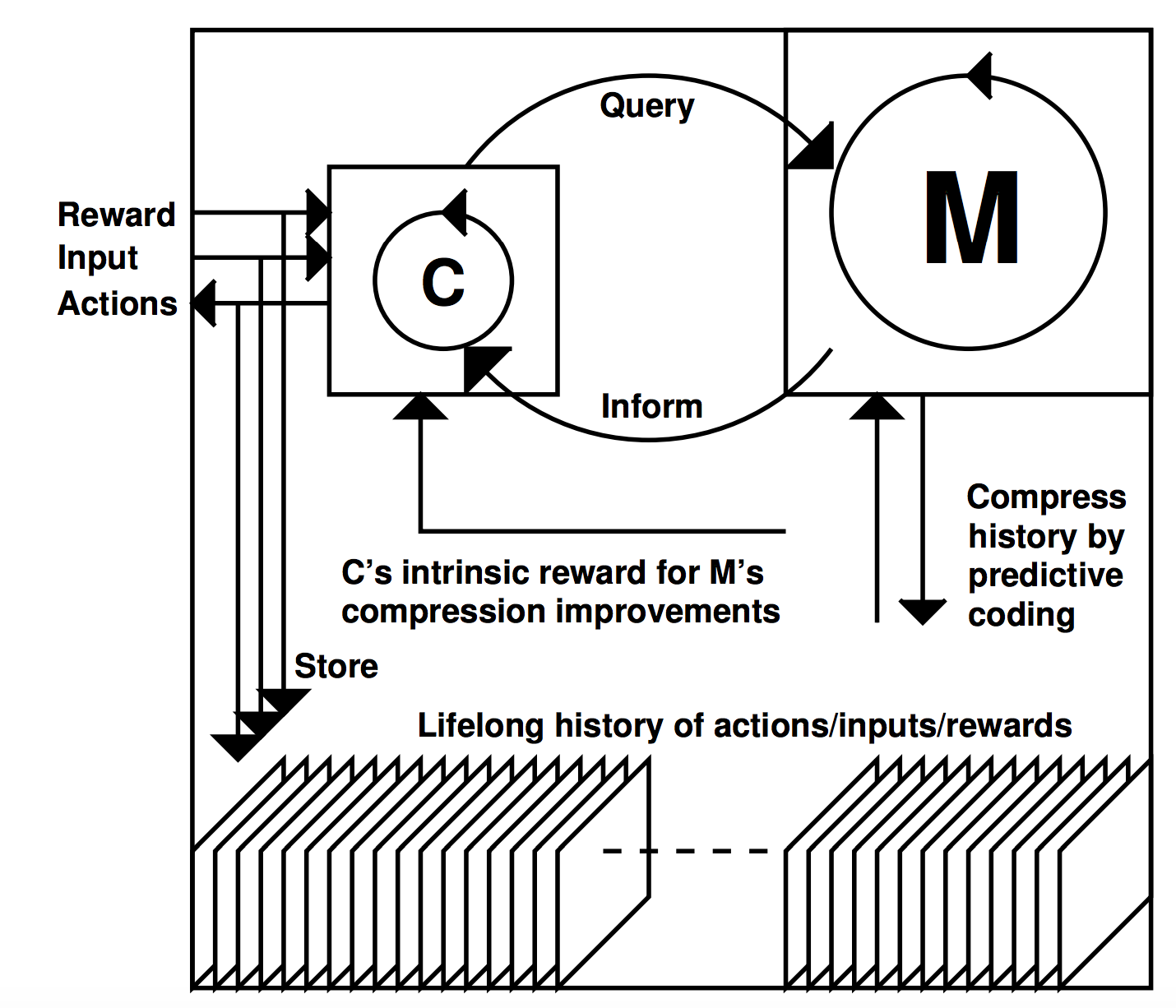
Figure 1: In a series of trials, an RNN controller C steers an agent interacting with an initially unknown, partially observable environment. The entire lifelong interaction history is stored, and used to train an RNN world model M, which learns to predict new inputs from histories of previous inputs and actions, using predictive coding to compress the history (Sec. 4). Given an RL problem, C may speed up its search for rewarding behavior by learning programs that address/query/exploit M’s program-encoded knowledge about predictable regularities, e.g., through extra connections from and to (a copy of) M—see Sec. 5.3. This may be much cheaper than learning reward-generating programs from scratch. C also may get intrinsic reward for creating experiments causing data with yet unknown regularities that improve M (Sec. 6). Not shown are deep FNNs as preprocessors (Sec. 4.3) for highdimensional data (video etc) observed by C and M.
This series of posts will delve into the different ways of connecting C and M together. Unfortunately, the paper does not enumerate a lot of such ways.
In section 5.3:
Consider an RNN C (with typically rather small feasible search space) as in Sec. 5.2. We add standard and/or multiplicative learnable connections (Sec. 3.1) from some of the units of C to some of the units of the typically huge unsupervised M, and from some of the units of M to some of the units of C. The new connections are said to belong to C. C and M now collectively form a new RNN called CM, with standard activation spreading as in Sec. 3.1.
The activations of M are initialized to default values at the beginning of each trial. Now CM is trained on RL tasks in line with step 3 of algorithm 1, using search methods such as those of Sec. 5.2 (compare Sec. 1). The (typically many) connections of M, however, do not change—only the (typically relatively few) connections of C do.
Later in 5.3:
Numerous topologies are possible for the adaptive connections from C to M, and back. Although in some applications C may find it hard to exploit M, and might prefer to ignore M (by setting connections to and from M to zero), in some environments under certain CM topologies, C can greatly profit from M.
Having introduced the main ideas of the paper, we are ready to consider the different ways C and M can interact together. This will be the subject for part 2.
In the meantime, I’ll just end this part with a wild speculation: This CM topology reminds me a bit about the human brain, where M is the neocortex and C the hypocampus and/or thalamus.